Wholesale Credit
Risk Engine.
A full PD → LGD → EAD → portfolio-loss stack built on a genuine low-default portfolio — 1.20% annualised, 692 defaults across 229,803 obligor-quarters. Firth-penalised logistic scorecard on monotone WoE bins, validated out of time, with conservative PD calibration for zero-default rating grades, and loss projected under both CCAR stress scenarios and a CECL lifetime expectation.
Every obligor, financial ratio, facility, default event, realised LGD and realised CCF in this project is simulated. No real borrower data is used anywhere. Only the macro factor is real, pulled live from FRED. The project demonstrates modelling and validation method; the numbers describe a simulated portfolio and support no inference about any real credit book.
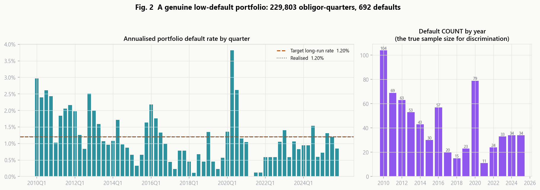
Everything here follows from one fact.
A wholesale credit book is a low-default portfolio. This one defaults at 1.20% a year: 692 events in 229,803 obligor-quarters, and only 136 out of time. The single most useful thing to internalise about PD modelling is that the effective sample size is the number of defaults, not the number of rows. Almost every technique on this page is a response to having very few events.
| Consequence of few defaults | What the model does about it |
|---|---|
| Discrimination statistics are noisy | Bootstraps the Gini and displays the interval |
| Logistic MLE is biased, can fail to converge | Firth's penalised likelihood |
| Some grades have zero observed defaults | Jeffreys prior, with Pluto‑Tasche as benchmark |
| Defaults cluster in time | Out‑of‑time split, never random |
| Rows from one obligor aren't independent | Obligor‑clustered bootstrap |
Real macro, synthetic obligors.
Four series are pulled live from FRED and collapsed into a single standardised credit-cycle index Z (higher = worse). Equal weights on the sign-oriented standardised series — deliberately not a fitted PCA, because fitted weights on 64 quarterly observations would be close to pure noise. If no API key is present, each series falls back to a calibrated synthetic analogue and the mode used is reported per-series in the console, in the figure below, and in the model document header.
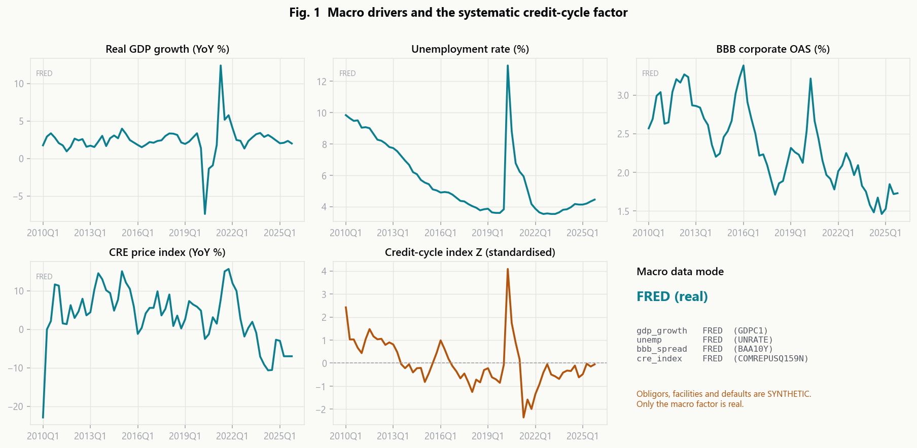
Z. The index peaks at +4.1σ in 2020Q2, with the GFC hangover (2010Q1) and the euro crisis (2011Q3) as secondary stress.Two data traps, both easy to miss
- The obvious BBB spread series,
BAMLC0A4CBBB, only carries about three years of history on FRED — useless for a 2010–2025 panel. Replaced withBAA10Y(Moody's Baa less the 10-year Treasury), daily from 1986. COMREPUSQ159Nis already published as a year-on-year growth rate. Differencing it again produced values in the hundreds of percent. Caught by looking at the raw series rather than trusting the series name.
How defaults are generated
A one-factor Merton/Vasicek latent-variable model. An obligor defaults when its latent asset index crosses a threshold:
A = √ρ · Z · βsector + √(1−ρ) · [ a·s + √(1−a²)·e ], default if A > k.
s is a creditworthiness index over the five financial ratios; a = 0.36 is the share of idiosyncratic variance those ratios explain, which is what sets attainable discrimination; ρ = 0.16 is asset correlation, inside the Basel corporate range. k is solved by bisection to hit 1.20% annualised on the surviving panel — default is absorbing, so obligors exit, and calibrating on the pre-exit grid is simply wrong.
One judgement call worth defending
The real macro stress index hits +4.1σ in 2020Q2. Fed straight into a Vasicek model, that implies a quarterly default rate around 10% — roughly 40% annualised. That is not what happened. Corporate default rates in 2020 rose to a few multiples of normal, not forty, largely because policy support broke the historical macro-to-default relationship. The factor is therefore tanh-squashed: linear through the ordinary range, compressed in the tail. 2020 and the 2010–11 hangover remain clearly the worst periods in the sample, at roughly 3× the long-run rate.
Weight of Evidence, then Firth.
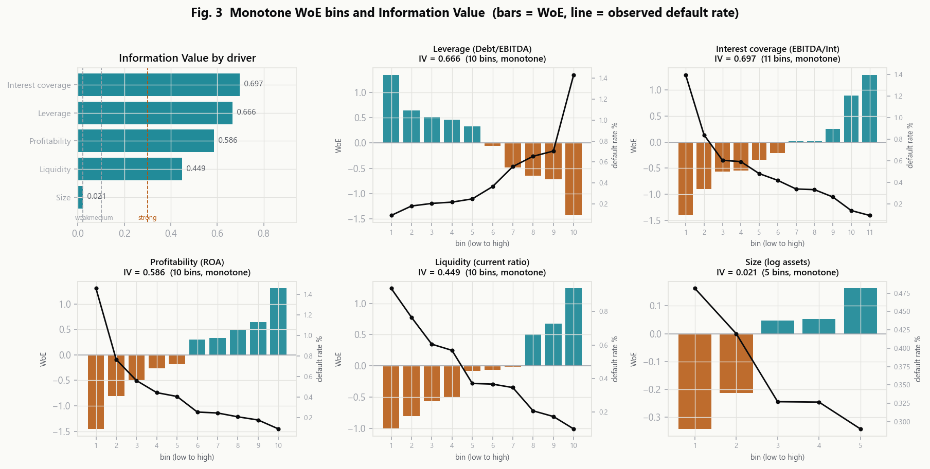
Each continuous driver is binned, and each bin gets WoE = ln(%non‑default / %default), so a higher WoE means safer. Binning linearises a non-linear driver-to-log-odds relationship without letting the model invent an arbitrary shape; it is robust to the outliers that dominate financial ratios (a 40× leverage observation stops being a leverage point); and it makes the scorecard readable, because every rating decomposes additively into a per-driver contribution a credit officer can challenge.
A credit officer will not sign off on a model in which more leverage lowers PD over some interval, regardless of how well it fits. Bins are quantile-seeded and then adjacent bins are merged until the default rate is monotone in the policy-mandated direction. Enforcing it up front is cheaper than explaining it later to model risk management.
The bit most implementations get wrong
Bins need a minimum number of defaults, not just a minimum number of observations. Without that constraint, quantile seeding leaves bins holding zero or one default; the smoothed WoE for such a bin is an artefact of the smoothing constant rather than an estimate, and Information Value comes out inflated by an order of magnitude. My first run produced IVs of 6.4 — that was the bug, and tying the minimum to a fraction of the total default count rather than the observation count is what fixes it.
| Driver | Information Value | Bins | Reading |
|---|---|---|---|
| Interest coverage (EBITDA/interest) | 0.697 | 11 | above the 0.50 caution line |
| Leverage (Debt/EBITDA) | 0.666 | 10 | above the 0.50 caution line |
| Profitability (ROA) | 0.586 | 10 | above the 0.50 caution line |
| Liquidity (current ratio) | 0.449 | 10 | strong |
| Size (log assets) | 0.021 | 5 | weak, retained |
The top three exceed 0.50, and by convention that is a leakage warning. Worth saying before anyone else does: here it is an artefact of the synthetic process, because the ratios literally generate the latent default index, so their relationship to default is cleaner than any real accounting ratio's would be. Note also that IV is a univariate screen and does not add up across correlated drivers — which is why individual IVs near 0.7 sit comfortably alongside a portfolio Gini of 0.59.
Champion: Firth-penalised logistic regression
Firth adds a Jeffreys-prior penalty +½·log|I(β)| to the log-likelihood. Ordinary maximum-likelihood logistic regression is biased away from zero in rare-event samples and — the property that actually matters operationally — is not guaranteed to produce finite estimates under quasi-complete separation. On a low-default book, the first time you cut the sample by sector or vintage and hit a cell with no defaults, plain MLE diverges. A model that silently blows up on a thin sector cut cannot be run in production. Implemented from scratch by modified-score iteration.
Out of time, never random
Train on quarters before 2021Q1; test from 2021Q1 on. A random split would put observations from the same stressed quarter on both sides. Because defaults cluster in time — and that clustering is the systematic factor — a random split lets the model see the realised cycle it is being asked to predict, and inflates measured discrimination. Out-of-time is the only split that answers the question a supervisor actually asks: does this model still rank-order on a cycle it was not fitted to?
Grade 1 has zero defaults. Now what?
The score is cut into 10 grades on the development sample, and the cut points are then frozen and applied unchanged out of time — re-cutting on the test sample would conceal exactly the migration the PSI diagnostic exists to detect. The masterscale is deliberately not equal-population: fine at the safe end, coarse at the distressed end, like the S&P and Moody's scales. That is where rating decisions are made, and it means the safest grades carry few or zero defaults — the problem to handle, rather than hide.
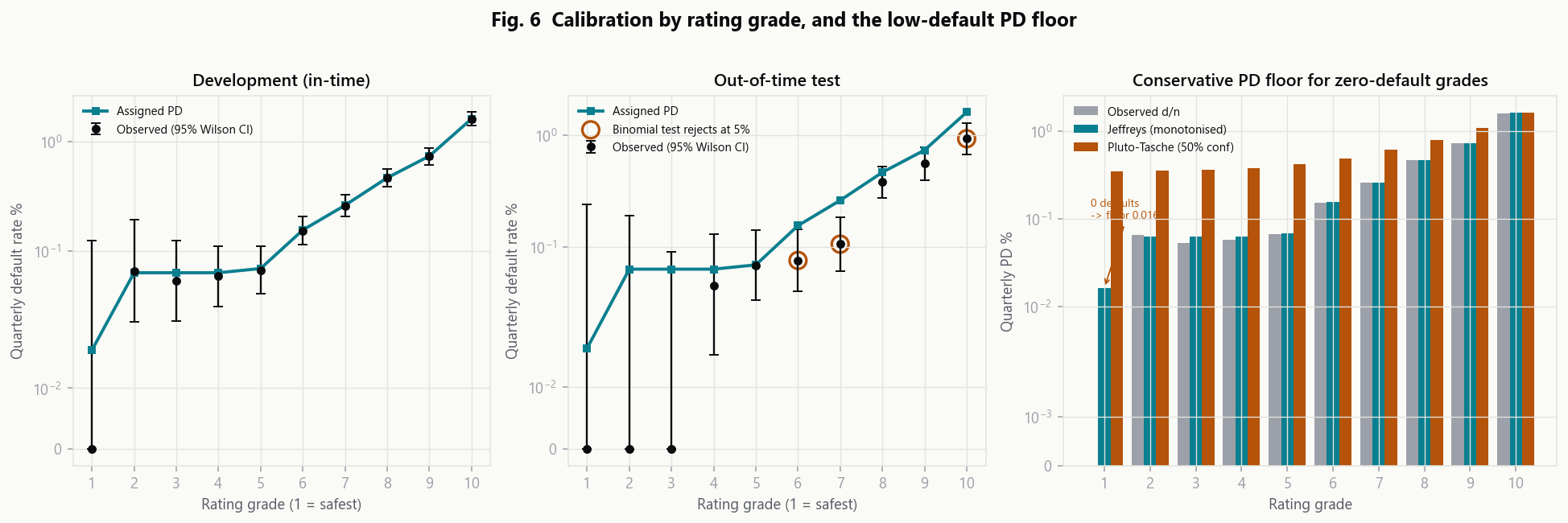
Grade 1 in this run holds 3,083 obligor-quarters and not one default. A naive d/n assigns PD = 0, and therefore zero capital and zero allowance. A zero is not an estimate; it is an absence of evidence.
Jeffreys posterior mean
(d + 0.5) / (n + 1)
On a zero-default grade this returns 0.5/(n+1) — strictly positive, shrinking sensibly as the grade population grows, and not contaminating neighbouring grades. Monotonised across grades by weighted isotonic regression, then floored at the Basel 3bp annual minimum. This is what is assigned.
Pluto‑Tasche most prudent
1 − (1−γ)^(1/N)
Pool grade g with every grade worse than g — valid under the rating ordering, which implies the least favourable configuration is equal PD across the pool — then take the upper confidence bound. Monotone in the grade by construction. Reported as a benchmark, not assigned.
"Assign the most prudent estimate" is the naive reading of the method. But for the safest grade, the Pluto‑Tasche pool is the entire portfolio, so its most prudent estimate is approximately the portfolio-wide default rate — in this run 0.34% per quarter against an assigned 0.016%, a factor of 21. Assigning it would rate the best obligors in the book at the average, fail the binomial calibration test across most of the scale, and drag the neighbouring grades up with it through the monotonicity constraint. That is a recognised criticism of the method, not an implementation detail. So it is used the way it is used in practice: as a conservatism benchmark and estimator of last resort.
The interval, not the point estimate.
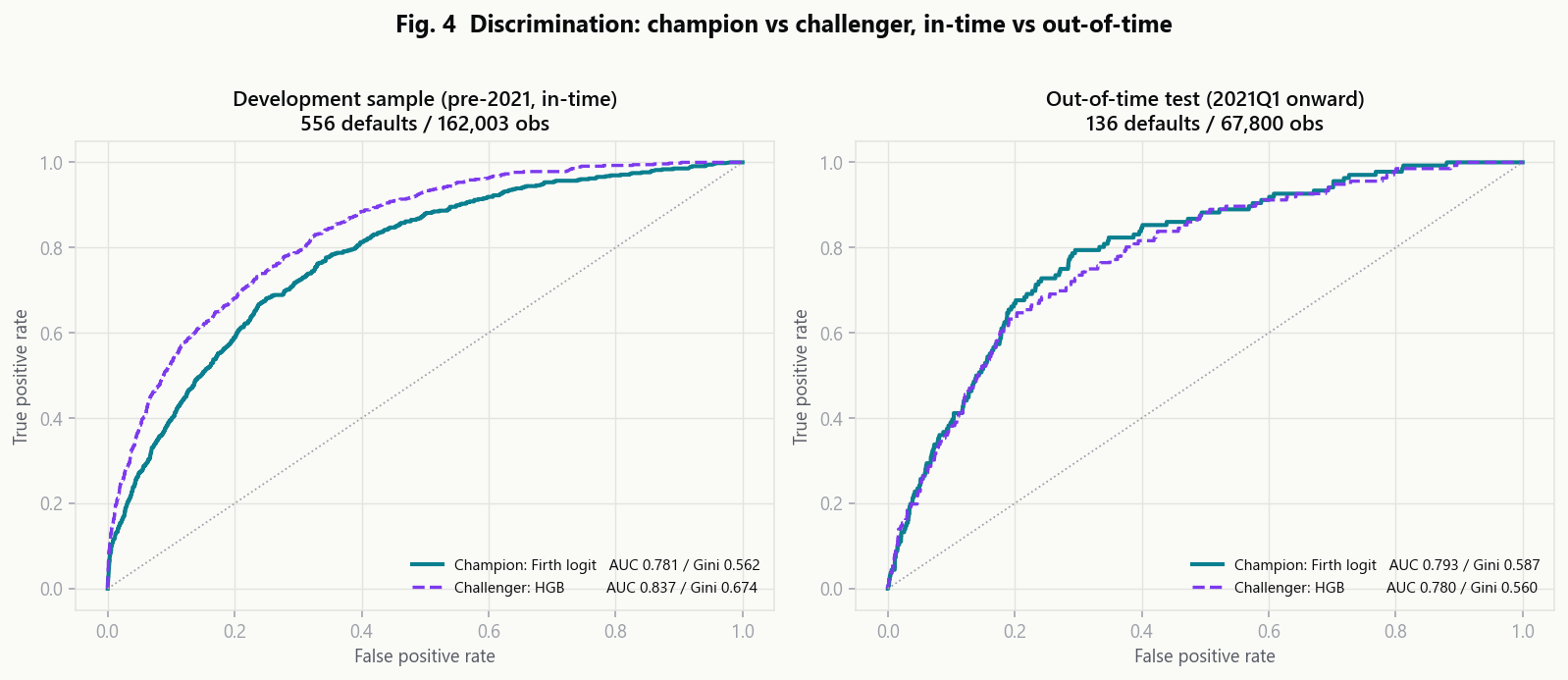
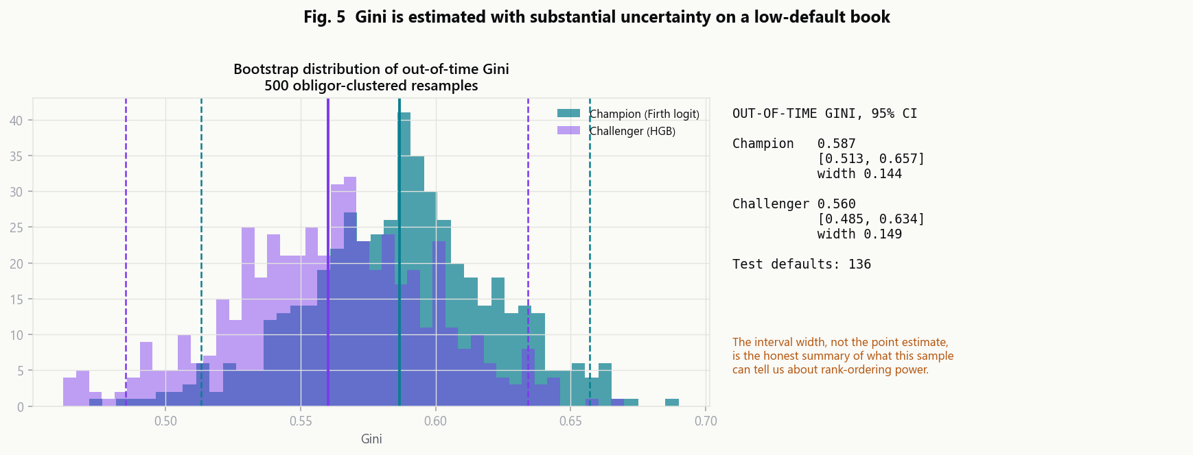
Out-of-time Gini 0.587, against a development Gini of 0.562 — so discrimination does not decay out of time. But the headline number is the 95% confidence interval: [0.513, 0.657], width 0.144.
With 136 out-of-time defaults you cannot resolve differences in Gini smaller than about 0.14. Reporting a Gini to three decimals on 136 defaults without the interval is the most common piece of quiet dishonesty in credit model validation. The bootstrap resamples obligors, not rows: consecutive quarters for the same obligor are not independent draws, so a naive row-level bootstrap reports a spuriously narrow interval — exactly the wrong direction for a diagnostic whose job is to convey uncertainty.
Stability
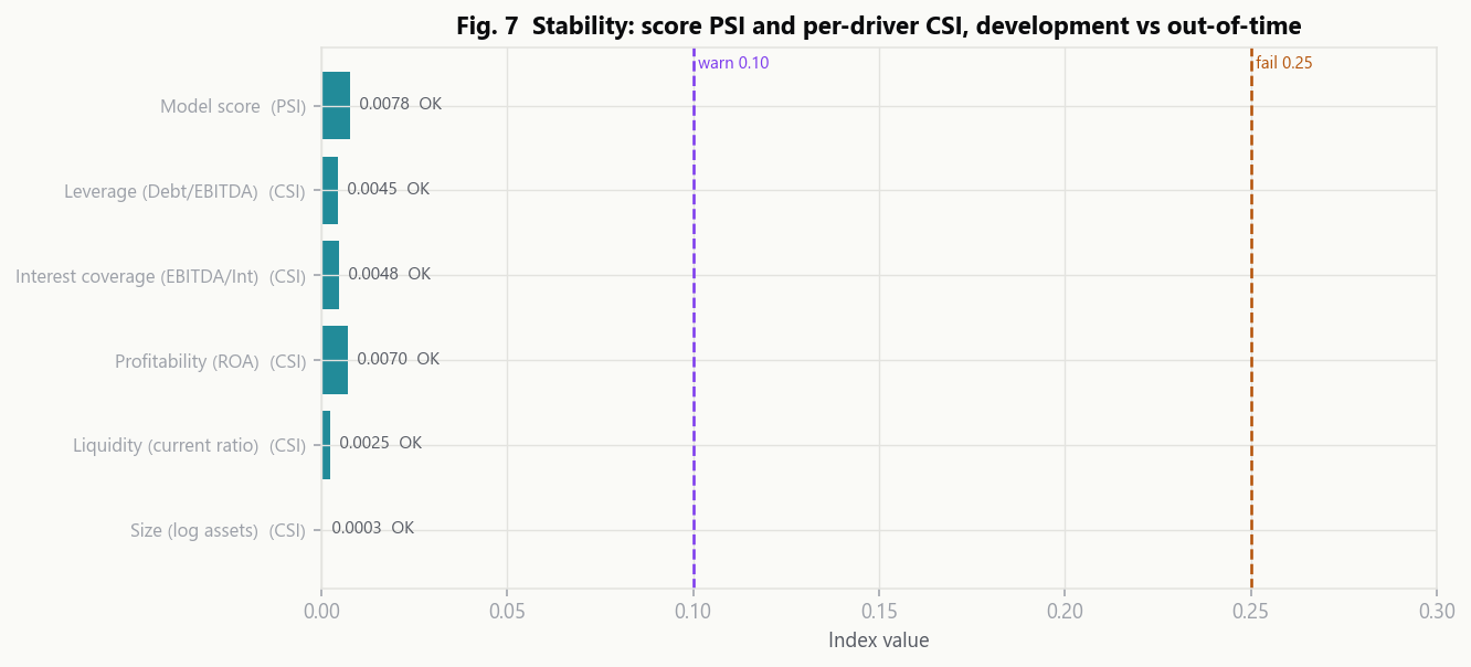
PSI on the score distribution and CSI per driver, development versus out-of-time, against the standard 0.10 amber / 0.25 red thresholds. Bins are cut on the development distribution and reused for the test sample — cutting separately returns approximately zero by construction, which is a real and common bug.
Champion versus challenger
| Metric | Champion — Firth logit | Challenger — HGB |
|---|---|---|
| Gini, in-time | 0.562 | 0.674 |
| Gini, out-of-time | 0.587 | 0.560 |
| Gini drop, train → test | −0.025 | +0.114 |
| KS, out-of-time | 0.499 | 0.444 |
| 95% CI on out-of-time Gini | [0.513, 0.657] | [0.485, 0.634] |
| Extrapolates beyond training range | Yes — linear in WoE | No — piecewise constant |
| Coefficient-level explainability | Yes | Post‑hoc only |
The logistic is retained as champion. Three reasons, in order of weight:
- The difference does not survive sampling uncertainty. Paired bootstrap of the Gini difference: −0.026, 95% CI [−0.056, +0.002] — not distinguishable from zero. Promoting a challenger on a difference the data cannot resolve is model risk, not model improvement.
- Governance explainability. Six coefficients on monotone, policy-signed WoE bins. Every rating movement decomposes additively into a per-driver contribution. The challenger requires post-hoc attribution, which is an explanation of an explanation.
- Gradient boosting cannot extrapolate. Tree ensembles are piecewise constant: outside the training range of a driver, the prediction is flat. In stress testing the entire question is what happens when drivers move beyond anything in the training window. A model structurally incapable of responding to that is disqualified for the use case, whatever its in-sample discrimination.
Reason 3 is the one that ends the argument, and it is specific to stress testing.
Bounded, bimodal, and drawn down.
LGD is estimated with a fractional-response GLM — binomial family, logit link, quasi-maximum likelihood (Papke–Wooldridge), with HC0 heteroskedasticity-robust standard errors. The robust covariance is not optional: under QMLE the model's own information-matrix standard errors are inconsistent.
(i) LGD is bounded on [0,1]. OLS is unconstrained and will predict negative losses on well-secured senior facilities and losses above 100% in the tail. Every one of those has to be manually overridden — which means the model is being corrected by the person it was supposed to inform.
(ii) LGD is bimodal: a mass near 0 (recovered, well-secured) and a second mass around 0.6–0.9 (unsecured, or collateral that evaporated with the borrower). OLS fits the conditional mean of that distribution — a value that is itself rarely observed. The fractional logit assumes nothing about unimodality; it only requires E[y|x] = Λ(x'β) to be correctly specified, which is precisely the object expected loss needs.
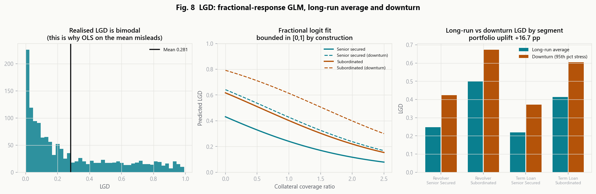
Downturn LGD is the same model evaluated with the macro stress term at its 95th historical percentile, holding facility characteristics fixed — the Basel "downturn conditions" idea without inventing a separate dataset.
EAD = drawn + CCF × undrawn
The regulatory question is how much of an undrawn commitment a borrower pulls down on the way to default. Estimated CCF is 0.519 for revolvers and 0.302 for term loans — but the operative result is the gradient across obligor deterioration.
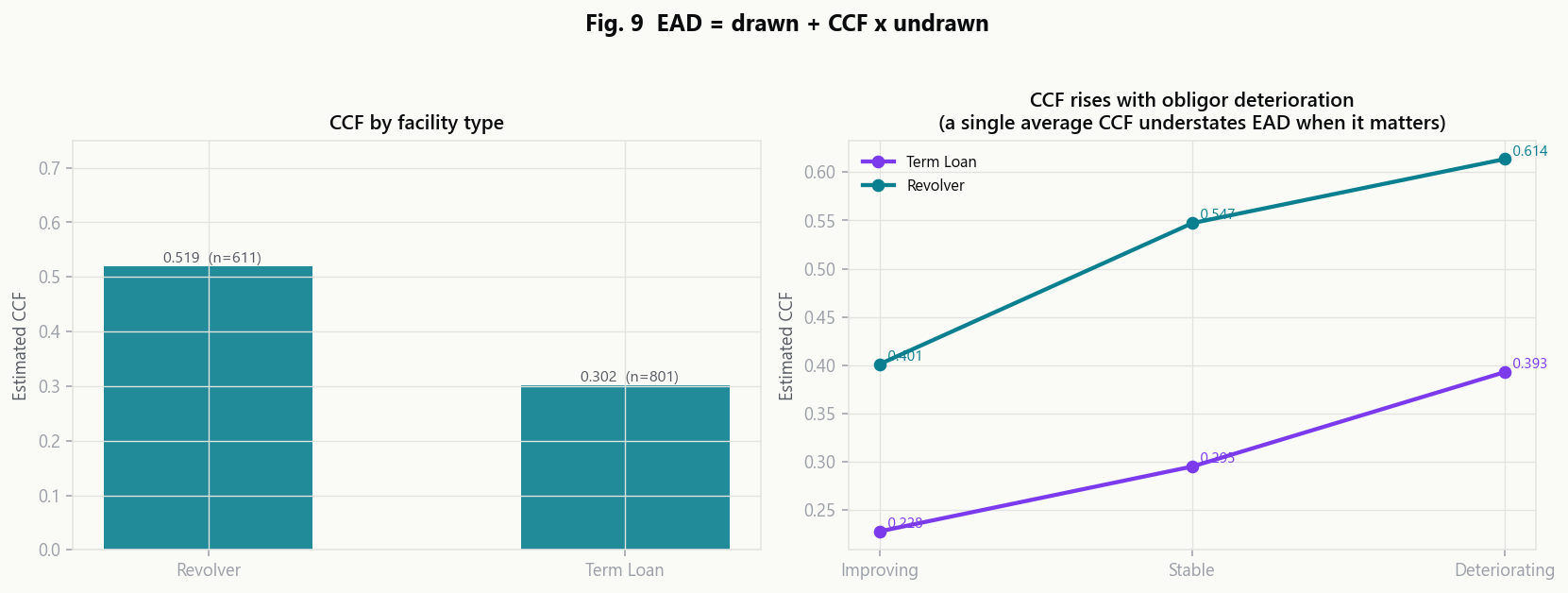
Obligors heading toward default draw on committed lines while they still can. A single portfolio-average CCF therefore understates EAD precisely in the states of the world where EAD matters. That sentence is the whole point of the module.
CCAR and CECL are not the same question.
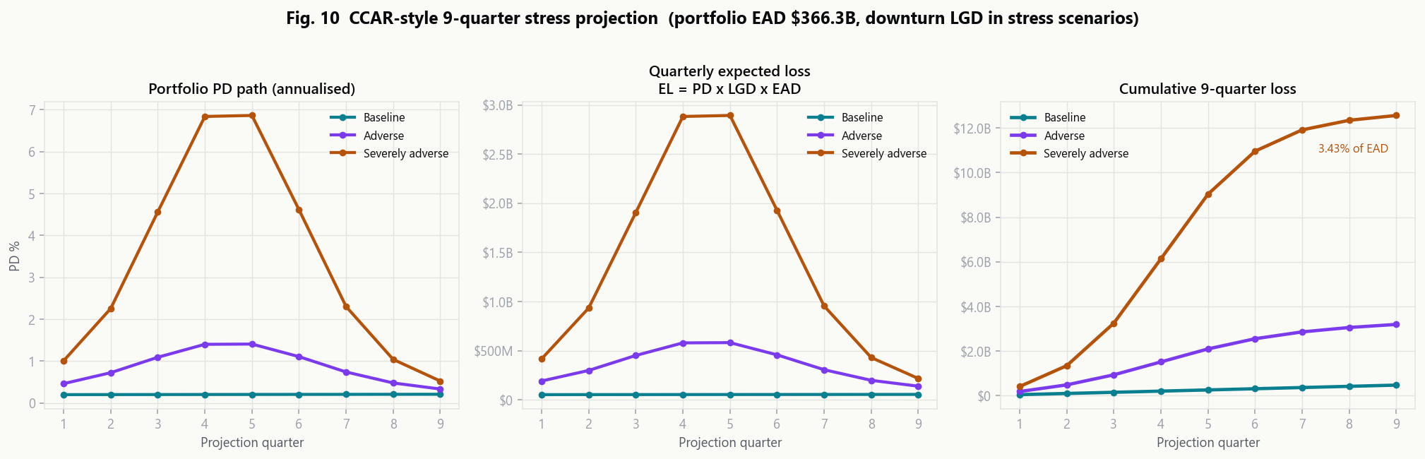
PD is conditioned on the macro state through the Vasicek single-factor transform, PD(Z) = Φ( (Φ⁻¹(PDttc) + √ρ·Z) / √(1−ρ) ). The asset correlation is moment-matched from the historical default-rate series (unconstrained estimate 0.083) and then bounded to the Basel corporate range, giving ρ = 0.12. The bridge from a supervisory macro path to Z is a four-variable OLS regression, R² = 0.66 — an ordering device, not a forecasting model.
My first run had the Vasicek inversion and the projection using opposite sign conventions, so the severely adverse scenario came out less risky than baseline. Worth checking explicitly that the stress scenario actually produces more loss than the baseline — an obvious sanity check that is easy to skip when the code runs cleanly and the plot looks plausible at a glance.
| CCAR / stress testing | CECL (ASC 326) | |
|---|---|---|
| Question | Losses on one prescribed supervisory path | Expected loss over remaining life |
| Horizon | Fixed 9 quarters | Lifetime of each exposure |
| Probability-weighted? | No — conditional on a path | Yes — an expectation |
| LGD basis | Downturn LGD (0.448) | Long-run average LGD (0.281) |
| Forecast | Given by the supervisor | 2‑year R&S forecast, then reverts to historical mean |
| Survival-adjusted? | No | Yes — an exposure defaults only once |
| The answer is | A conditional loss | A balance-sheet allowance |
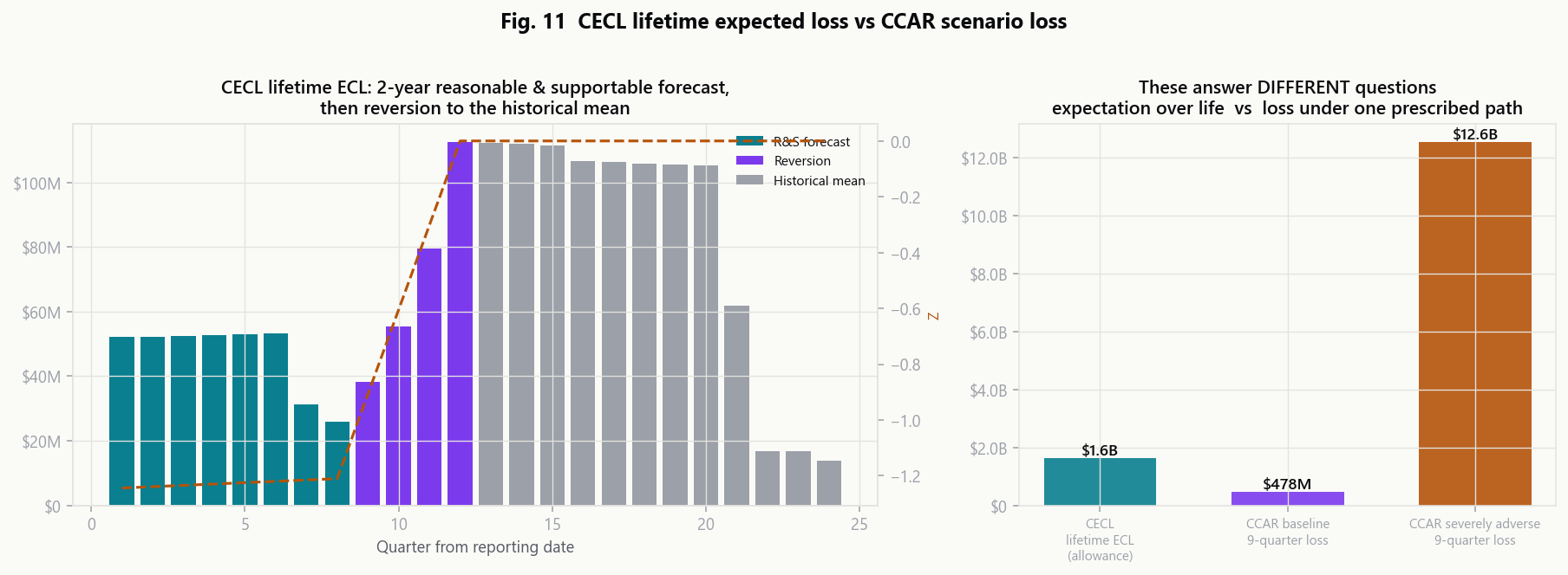
Z to zero, then the historical mean. Right panel: the two measures side by side — comparable as concepts, not as levels.| Measure | Loss | % of EAD |
|---|---|---|
| CCAR baseline, 9 quarters | $0.48B | 0.13% |
| CCAR adverse, 9 quarters | $4.55B | 1.24% |
| CCAR severely adverse, 9 quarters | $12.56B | 3.43% |
| CECL lifetime ECL (allowance) | $1.63B | 0.45% |
A model document that cannot drift.
The model document is generated from the run, not written by hand, so it can never fall out of step with the model. Its header stamps the semantic version, the git commit, the run timestamp and a SHA‑256 hash of the input data — change any input and the hash changes and the document changes with it. It is framed against SR 11‑7, the Fed/OCC supervisory guidance on model risk management. Two sections carry the weight.
§7 Limitations — deliberately blunt
- The obligor portfolio is synthetic, generated by a process close to the fitted form. Measured performance is an upper bound on what the same specification would achieve on real data.
- 692 defaults in total, 136 out of time. Every statistic downstream inherits that sample size.
- The out-of-time Gini interval spans 0.513 to 0.657. Any comparison turning on a difference smaller than that width is not supported by this sample.
- One realised cycle. The macro-to-
Zregression has four parameters on 64 quarterly observations, and should be treated as an ordering device rather than a forecasting model. - No qualitative overlay. Production rating systems apply analyst judgement, watchlist status, parent support and covenant breaches on top of the statistical score. None of that is here.
- No out-of-time validation of LGD or CCF. Both are estimated on the pooled defaulted population; there are too few defaults to hold out a time window and retain a usable sample. A genuine gap, not a simplification.
- Asset correlation is bounded, not freely estimated. The unconstrained estimate is 0.083 and was clipped into the Basel range. The clip is a judgement call and it moves the scenario losses.
§8 Monitoring thresholds — pre-committed
These are committed at development, before any monitoring result is observed. That ordering is the entire point: a threshold chosen after seeing the outcome is not a control.
| Metric | Amber | Red | Action at red |
|---|---|---|---|
| Score PSI vs development | 0.10 | 0.25 | Full revalidation; suspend for new rating assignment |
| Driver CSI, any single driver | 0.10 | 0.25 | Re‑bin that driver; reassess the WoE map |
| Gini fall vs development (0.562) | −0.10 | −0.15 | Full redevelopment |
| Grades failing binomial calibration | 2 of 10 | 3 of 10 | Recalibrate grade PDs; masterscale review |
| Realised vs assigned default rate | 1.5× | 2.0× | Recalibrate; escalate to credit risk committee |
| Observed vs long-run LGD (0.281) | +5pp | +10pp | Refit LGD; review downturn add‑on adequacy |
| Realised vs applied CCF | +5pp | +10pp | Refit CCF; review EAD on undrawn commitments |
| Age since last full validation | 12 months | 24 months | Mandatory revalidation regardless of performance |
Cadence: PSI and CSI monthly; discrimination and calibration quarterly on a rolling four-quarter window; full revalidation annually or immediately on any red breach. Escalation at red is written notification to model risk management within five business days, with a remediation plan and an interim compensating control — typically a conservative PD floor or an override requirement — in place until remediation completes.
Under 60 seconds, bit-reproducible.
The whole pipeline runs end to end in about 25 seconds warm and 37 seconds cold, on numpy, pandas, scikit-learn, statsmodels and matplotlib. No xgboost — the challenger is sklearn's HistGradientBoostingClassifier. Every stochastic component derives from one master seed via fixed per-module offsets, so adding a module cannot perturb an earlier module's draws.
The FRED key is read from the FRED_API_KEY environment variable and is never written to disk or committed; responses are cached locally so reruns skip the network. Without a key, every series falls back to a calibrated synthetic analogue and the mode used is reported per-series in the console, in Fig. 2, and in the model document header. You are never left guessing which data produced the numbers.
EXPLAINER.md is a ten-minute plain-English walkthrough of every module and the reasoning behind each choice, including a section of likely questions and short answers. MODEL_DOCUMENT.md is the generated SR 11‑7 document with the full diagnostic tables.
License: MIT. Synthetic data throughout except the FRED macro series. Not investment advice, and not a validated production credit model — see §1 and §7 of the model document for intended use and limitations.