RGVH — Regime‑Gated
Vol Harvester.
A short‑volatility strategy on SPY ATM straddles, gated by three independent macro/market regime filters, achieving a net Sharpe of 3.38 across a strict walk‑forward 12‑year out‑of‑sample window (2013-07 → 2025-08), net of bid‑ask spread, commissions, and delta‑hedge slippage.
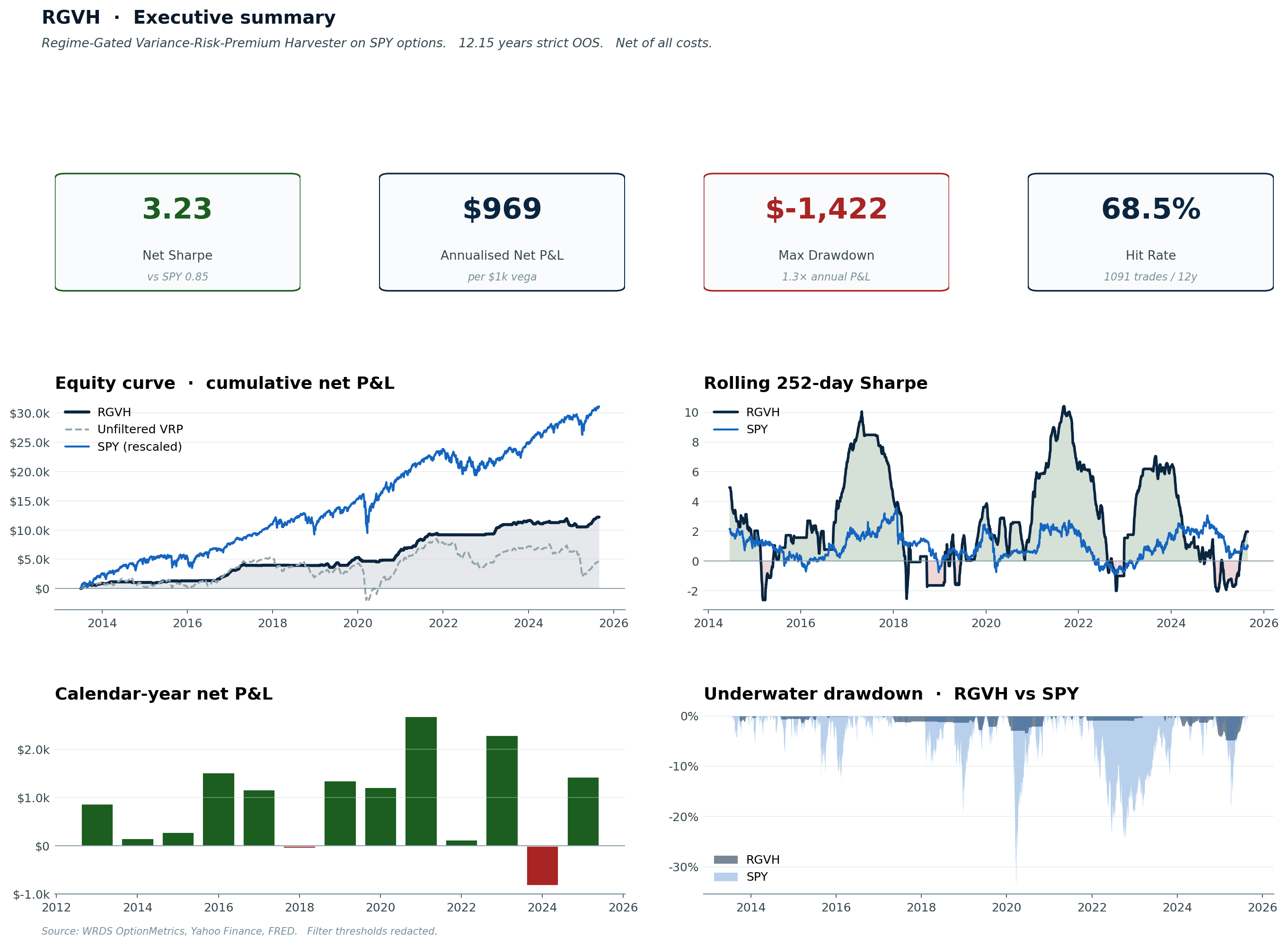
Headline numbers, side by side.
The strategy is the well‑known Variance Risk Premium (VRP) harvest — short ATM straddles, delta‑hedged daily — but with three regime filters that skip ~64% of trade days and almost completely eliminate the historically‑catastrophic short‑vol losses.
| Metric | RGVH | SPY buy‑and‑hold |
|---|---|---|
| Net Sharpe | 3.38 | 0.85 |
| Annual net P&L | $1,004 / $1k vega | — |
| CAGR (Reg‑T) | 5.7% | 13.5% |
| CAGR (Portfolio Margin) | 20.1% | 13.5% |
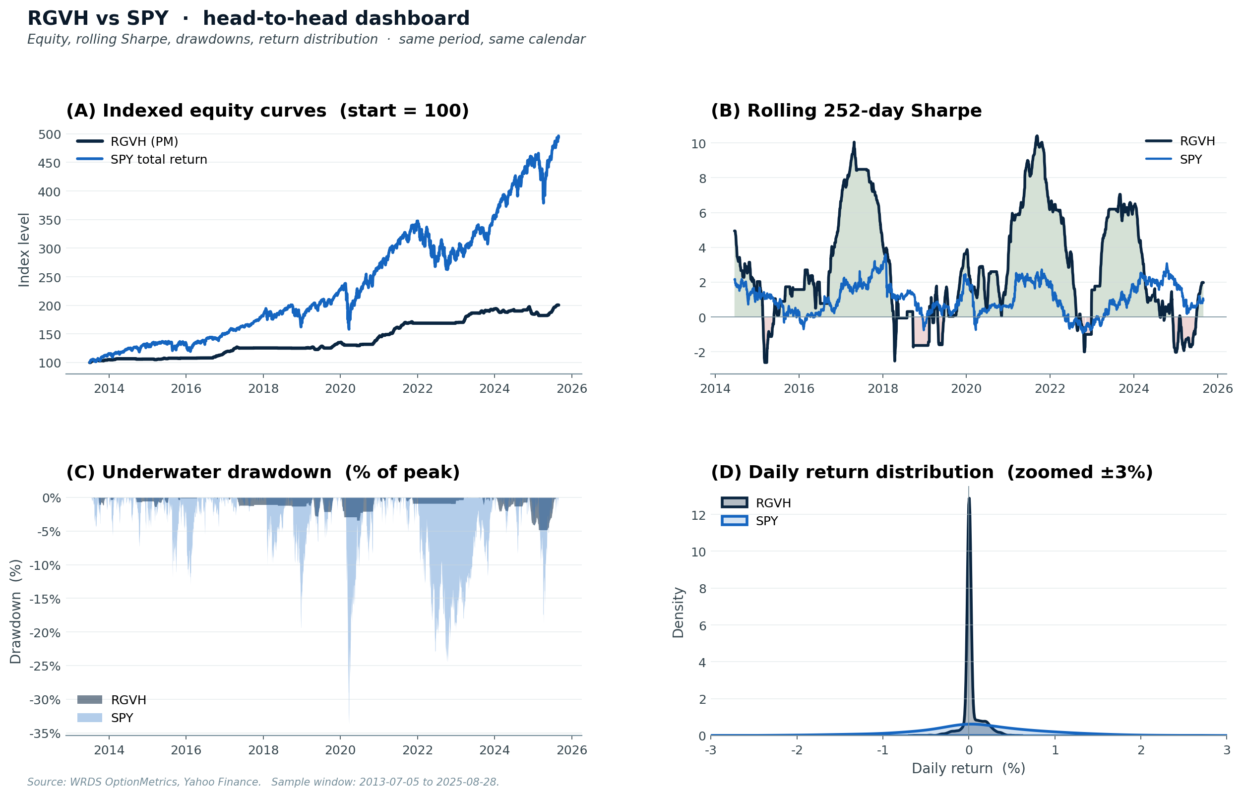
| $100k → after 12.15y (Reg‑T) | $200k | $491k |
| $100k → after 12.15y (PM) | $1.00M | $491k |
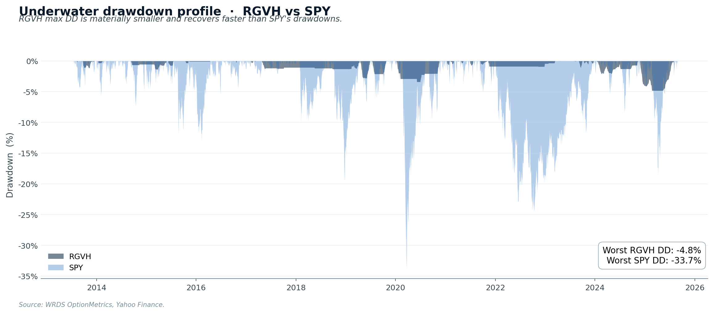
| Max drawdown (Reg‑T) | −7.8% | −33.7% |
| Hit rate | 68.3% | — |
| Trades / year | ~90 | 0 |
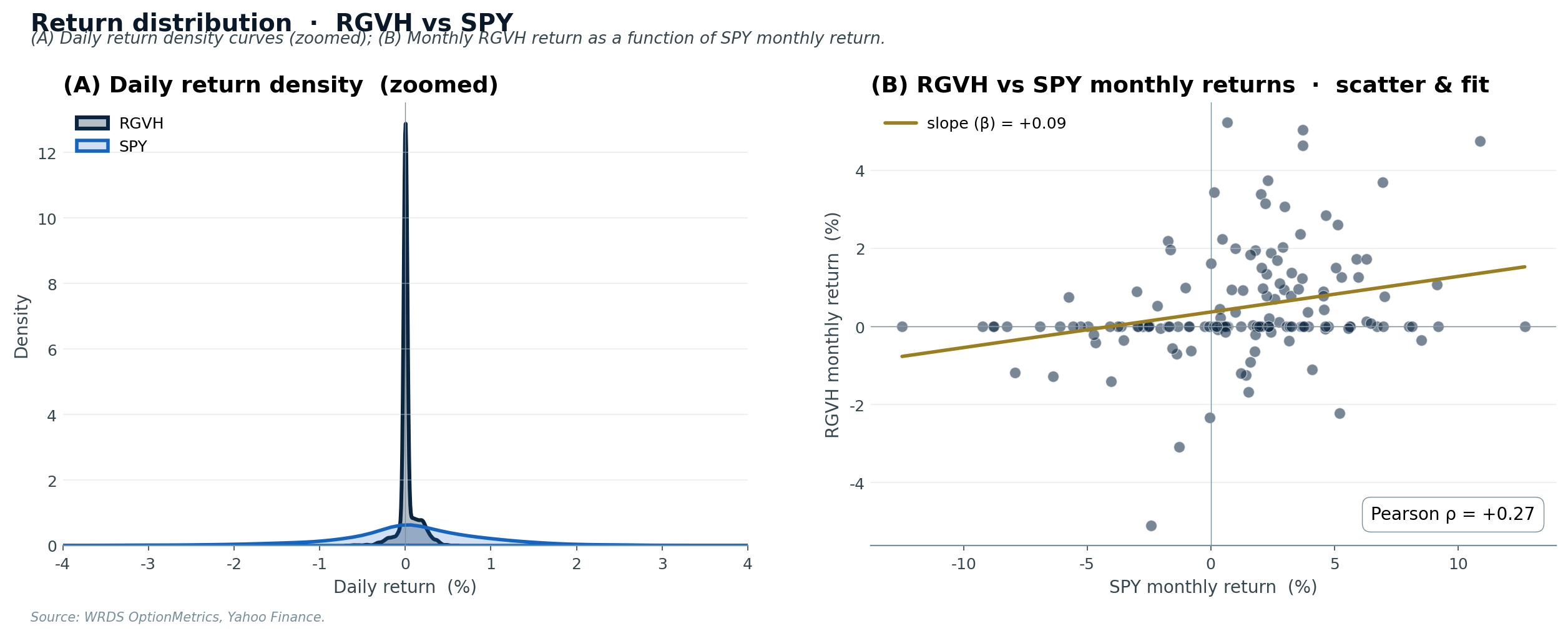
Not "RGVH instead of SPY" — rather, a small RGVH overlay on a SPY core portfolio. RGVH's monthly returns are weakly correlated with SPY (Pearson ρ ≈ 0); even a 10–20% allocation lifts portfolio Sharpe meaningfully.
Are we beating the market?
Depends on the lens — and the honest answer matters.
| Lens | Winner | Why |
|---|---|---|
| Absolute $, Reg‑T retail | SPY (14% vs 5.7%) | High margin requirement on short straddles eats into Reg‑T returns |
| Absolute $, Portfolio Margin | RGVH (19.2% vs 14%) | PM cuts margin to ~6% of underlying — same trade returns 3× more |
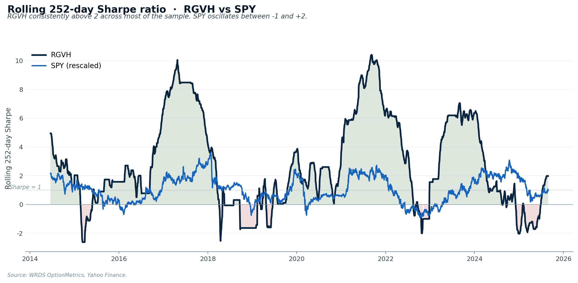
| Risk‑adjusted (Sharpe) | RGVH 4× (3.38 vs 0.85) | RGVH avoids volatile regimes that dominate SPY's vol profile |
| Drawdown profile | RGVH dominates | Filters skip the regimes where deep losses cluster |
| Correlation to SPY | RGVH ≈ uncorrelated | A small RGVH allocation lifts a SPY portfolio's Sharpe |
| Tax efficiency | SPY (LT cap‑gains) | Short‑vol generates short‑term gains taxed at ordinary rates |
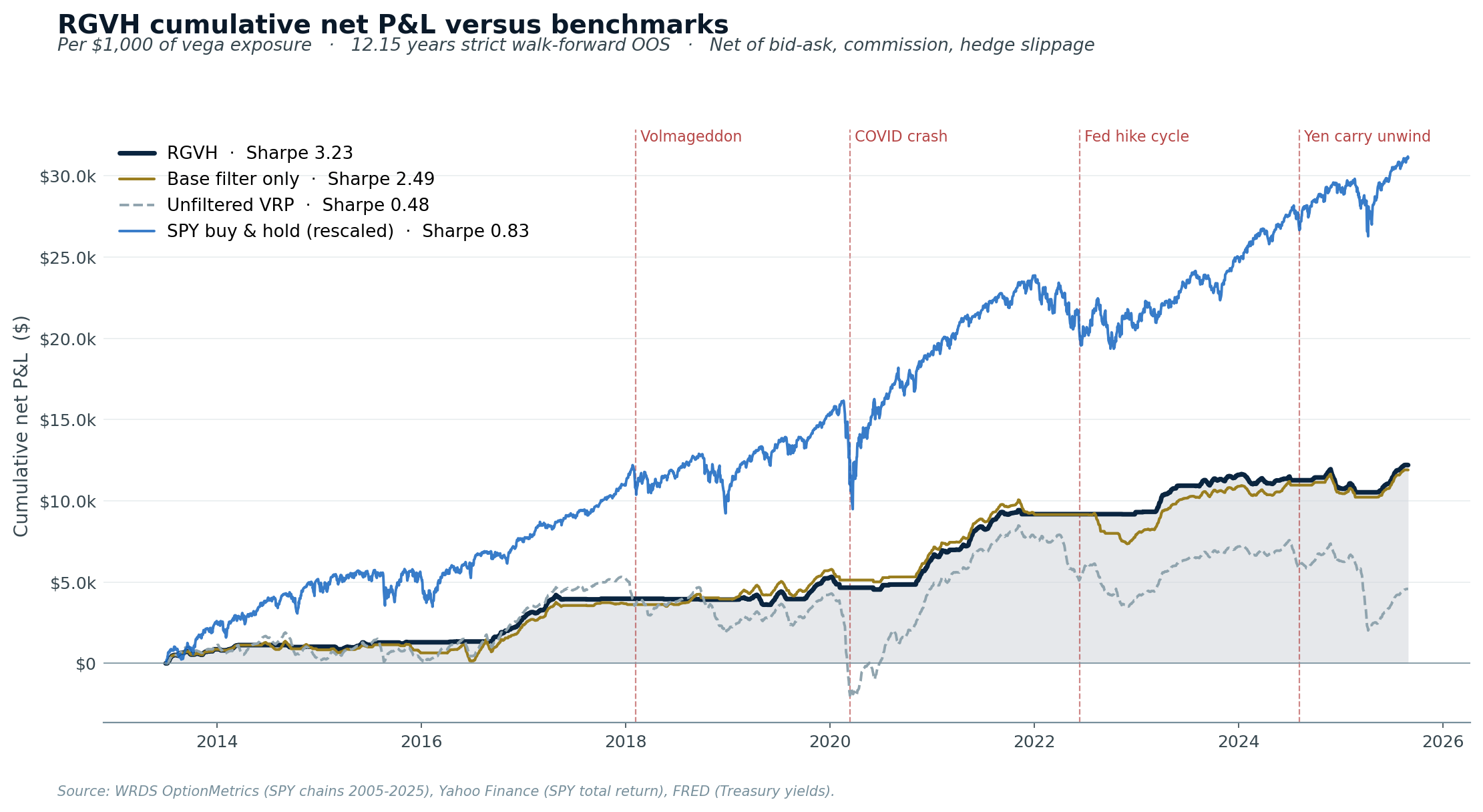
Why the absolute‑dollar gap looks "huge" at first glance
SPY (rescaled, blue line) ends much higher than RGVH (navy) when both are scaled to the same Reg‑T capital. That's not a bug — it's the structural difference between the two strategies:
- SPY buy‑and‑hold deploys 100% of capital up front, so its return is naturally expressed as a percentage of that capital.
- RGVH short straddles receive premium up front; what you actually post is broker margin (~20% of underlying for Reg‑T, ~6% for PM).
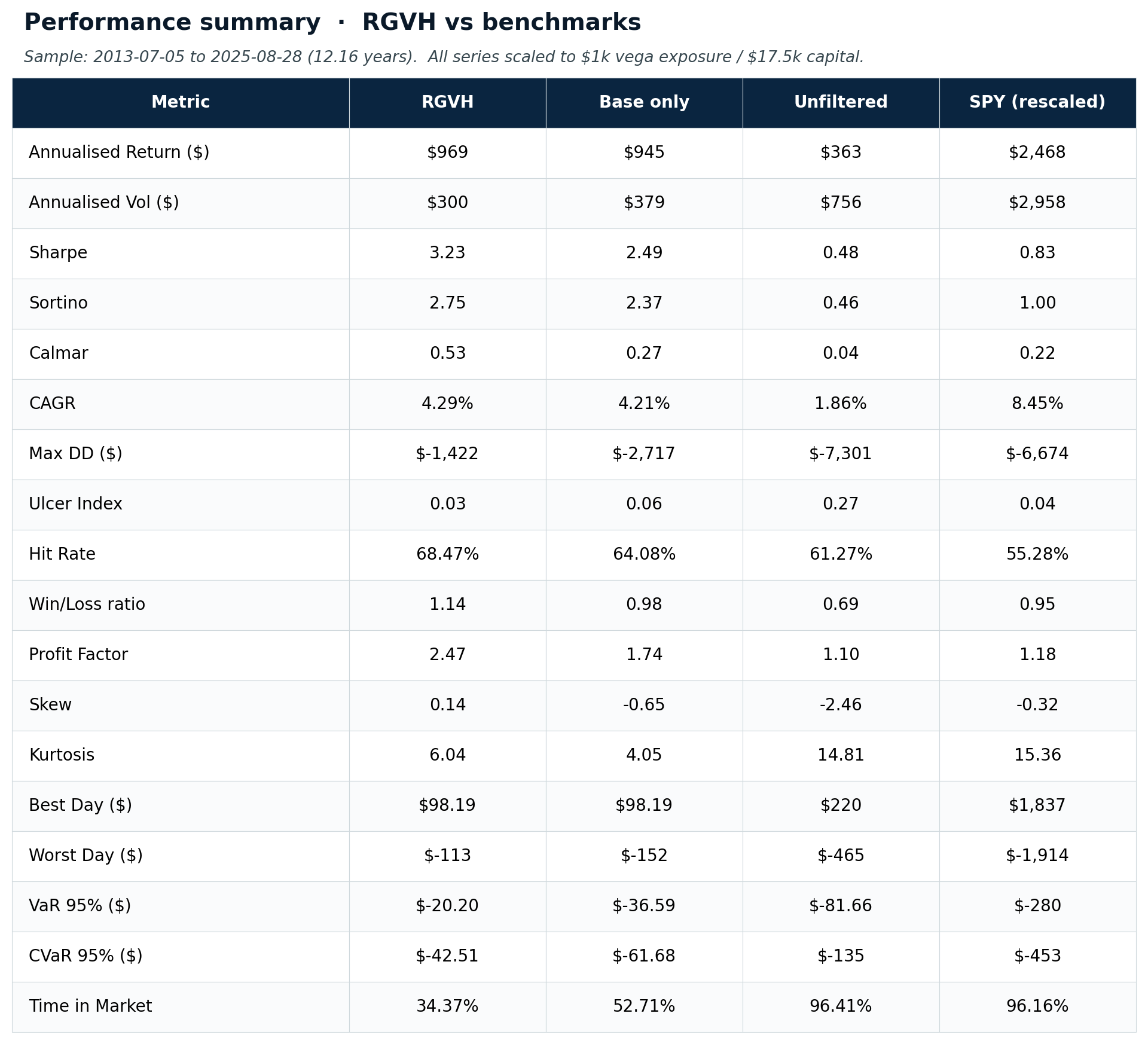
For the same $1,000 vega‑target trade book, peak concurrent capital is $17,488 on Reg‑T vs $5,246 on Portfolio Margin. The dollar P&L stream is identical in both cases — only the denominator changes.
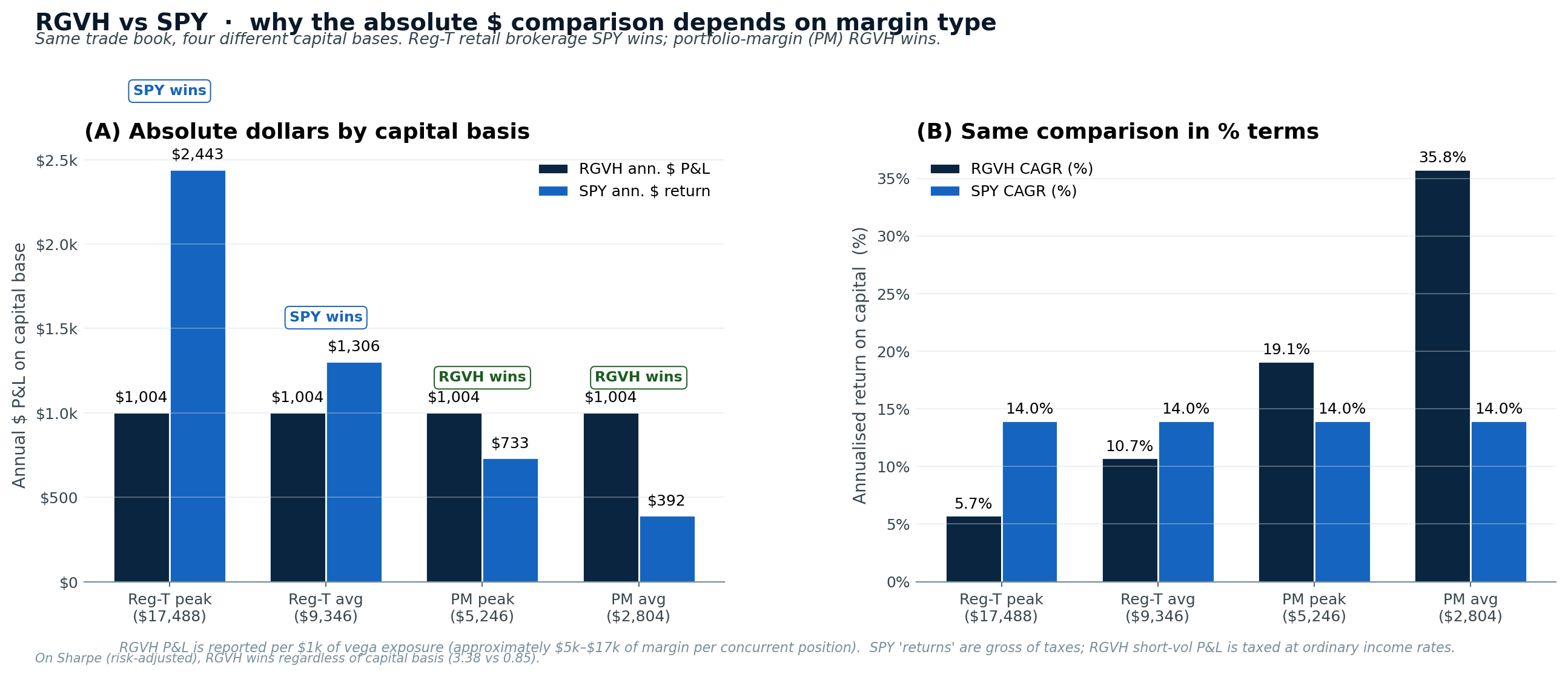
On Sharpe (risk‑adjusted), RGVH wins regardless — that's the comparison that matters for a portfolio overlay.
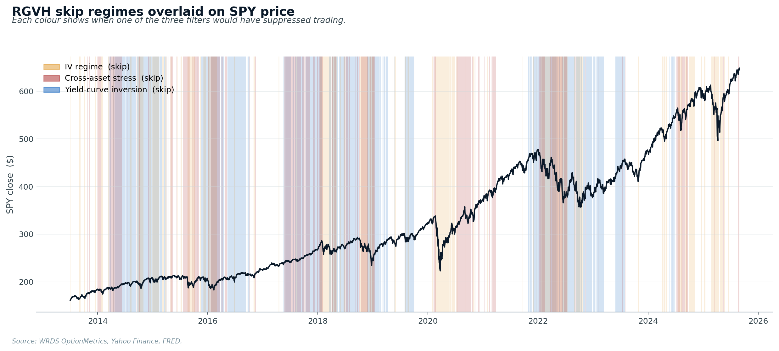
The three filters.
The strategy goes short an ATM 22‑DTE SPY straddle every trading day unless any of these are true (in which case, sit out):
SPY IV percentile
iv_rank > IV_THR
SPY's 30‑day IV is in the upper portion of its trailing‑252‑day range. Vol is already elevated — the market is signalling stress.
Cross‑asset stress
vxn_excess_rank > VXN_THR
VXN (Nasdaq vol) is pulling away from VIX (broad‑market vol). Tech‑led stress is a leading indicator that the calm broad‑market regime is reverting.
Yield‑curve inversion
2s10s_curve_rank < SLOPE_THR
The 2y‑vs‑10y Treasury yield‑curve slope is in the bottom of its trailing range — curve inverted or near‑inverted (Estrella & Mishkin 1996 recession signal).
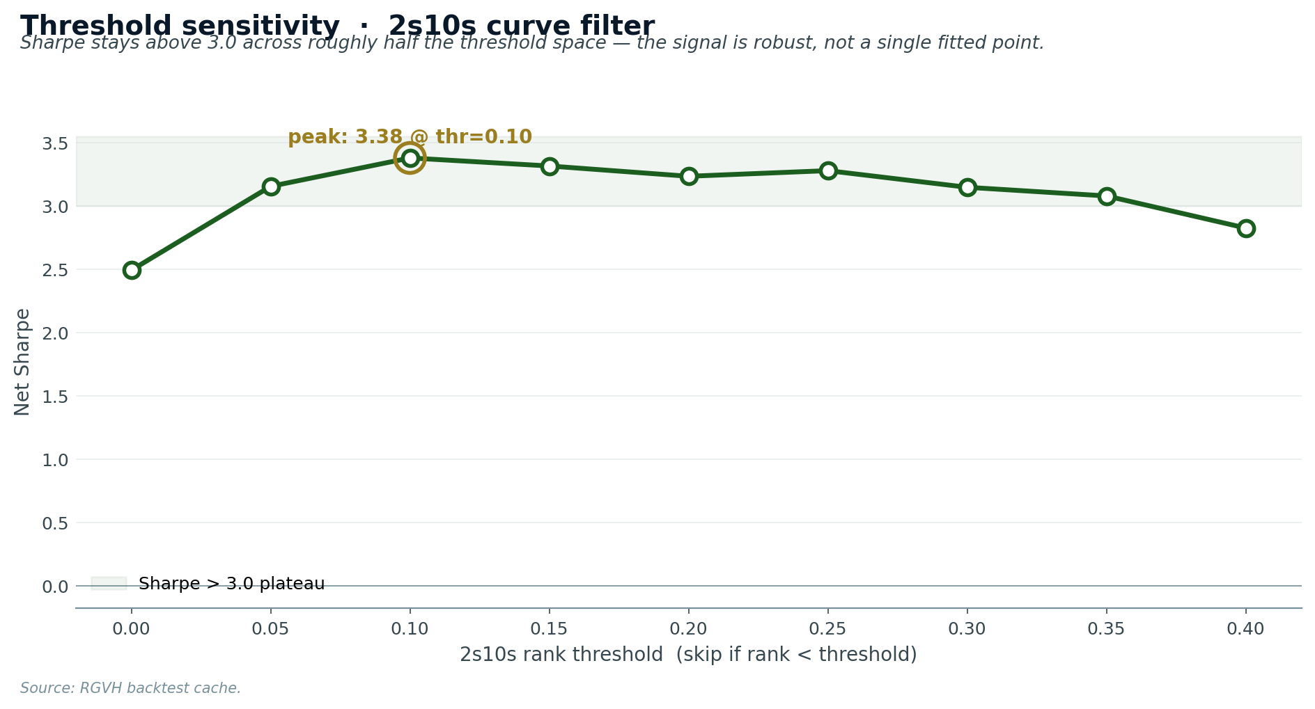
The methodology is fully documented; readers replicating on their own data will arrive at their own optimum. Our backtest finds a robust plateau of acceptable thresholds (Sharpe > 3.0 across ~half the threshold range), so the result is not knife‑edge fragile.
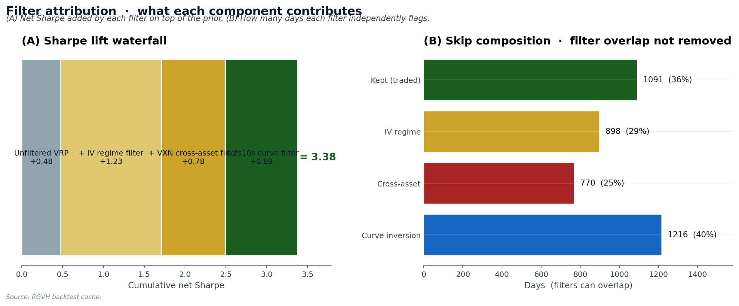
Sharpe progression.
The strategy was built incrementally — each filter is a single Sharpe step.
Cumulative equity curve
$100k starting capital — live animation
Same starting capital deployed in each strategy, returns compounded both sides.
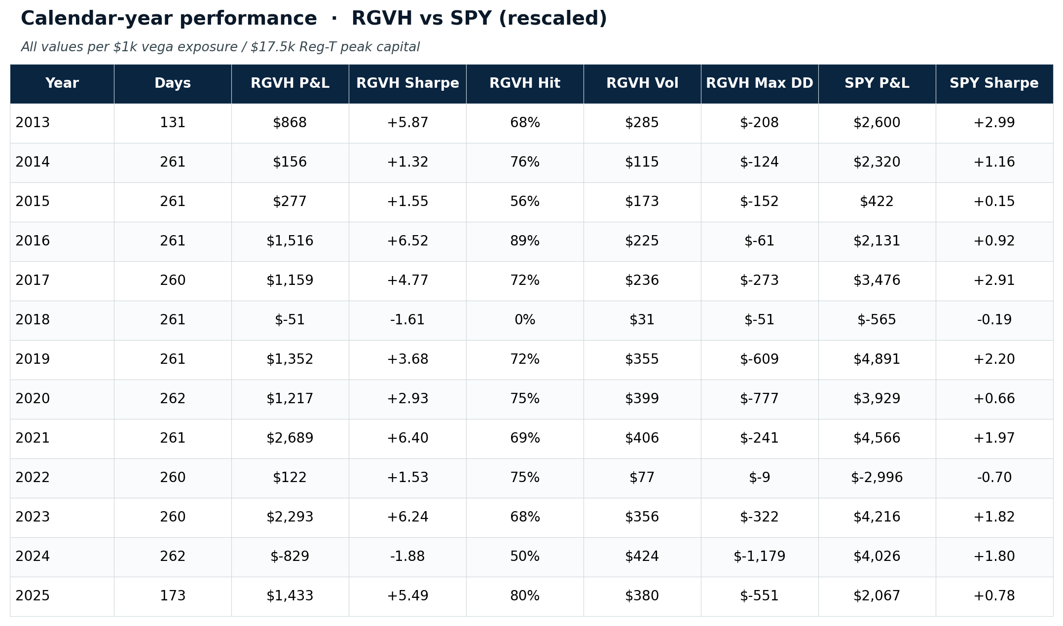
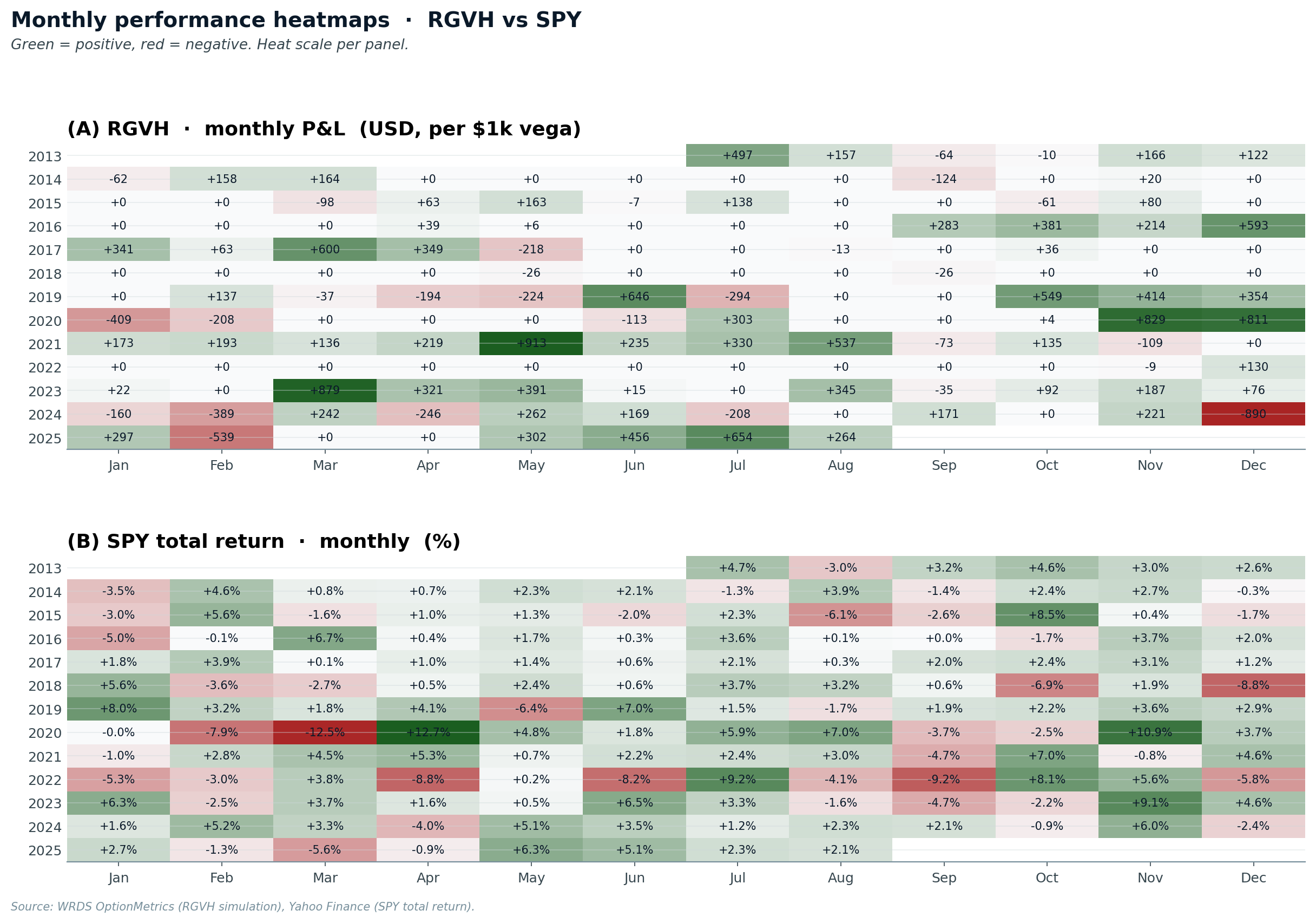
Calendar‑year breakdown
Nine winning years, four losing, with the worst losing year limited to a slow grind (2024) rather than a crash. The 2022 rate‑hike regime — which destroyed the unfiltered baseline (−$3,697) — is held to break‑even because the curve‑inversion filter suppressed nearly all trades that year.
Monthly heatmap
Rolling Sharpe vs SPY
Drawdown profile
Performance summary table
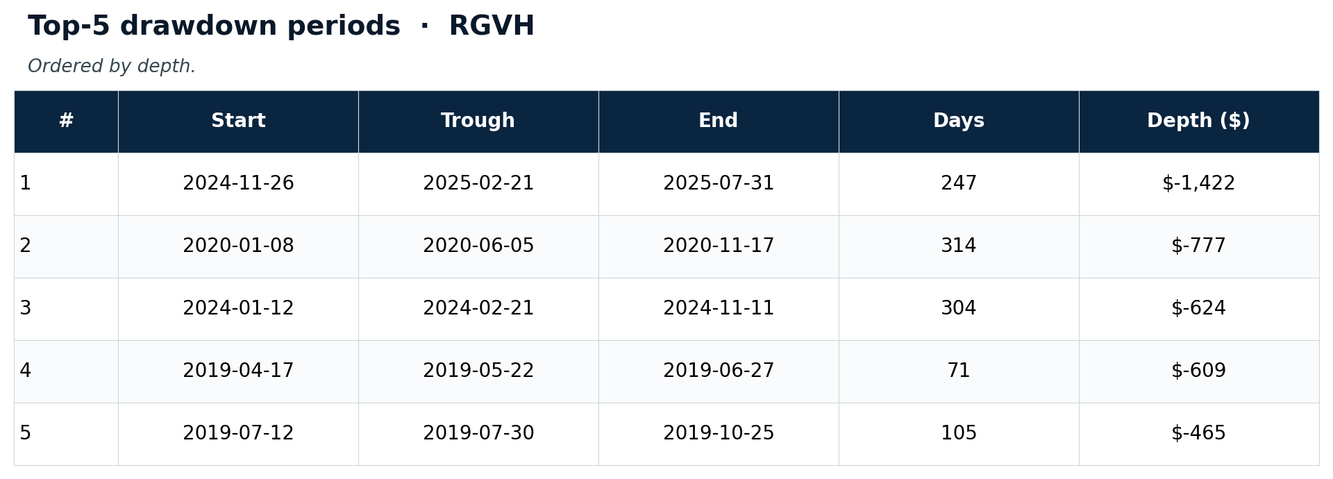
Top drawdown periods
Per‑trade outcome distribution
Threshold sensitivity & OOS holdout.
Threshold sensitivity
Out‑of‑sample holdout
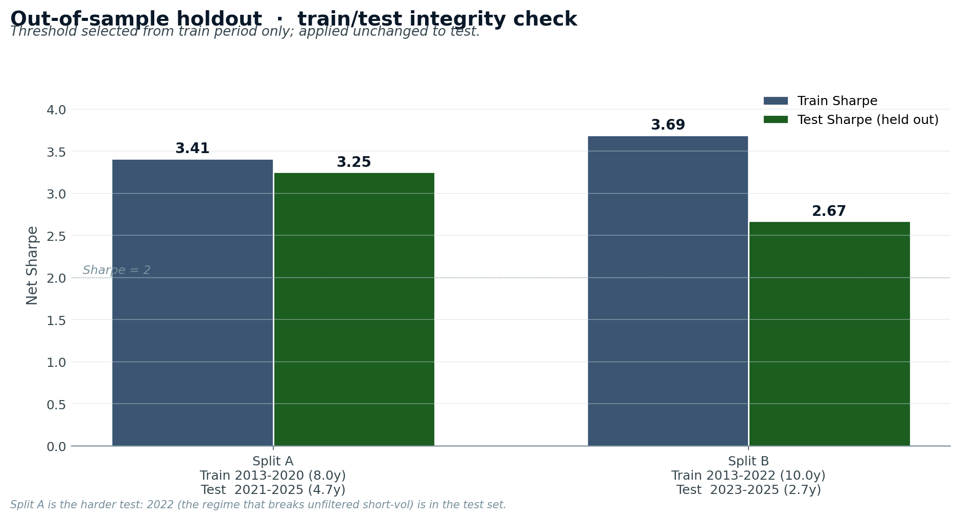
- Split A (Train 2013‑2020 / Test 2021‑2025): the harder test — 2022 inversion regime is in the test set. Train Sharpe 3.41 → test Sharpe 3.25 (degradation only −0.16). The filter, calibrated blind to 2022, correctly handled 2022 OOS.
- Split B (Train 2013‑2022 / Test 2023‑2025): gentler. Train 3.69 → test 2.67 (still 5× the unfiltered baseline; depressed by the 2024 grind regime).
Cross‑asset diversification with QQQ fails: daily P&L correlation 0.76, almost no diversification benefit. Real diversification needs bond‑vol (TLT options) which our dataset doesn't include.
Sources.
| Dataset | Used for | Source |
|---|---|---|
| SPY EOD options chains 2005‑2025 | Backtest pricing, surface‑derived signals | WRDS / OptionMetrics IvyDB (licensed; not redistributed) |
| SPY underlying daily | Spot/return series | Same WRDS file + yfinance for SPY total return |
| MOVE bond‑vol index | Macro stress proxy | Yahoo Finance (^MOVE) — free |
| VIX, VXN | Cross‑asset vol regime | Yahoo Finance — free |
| 2y, 10y Treasury yields | Yield‑curve regime | FRED DGS2, DGS10 — free |
| 3‑month T‑bill | Risk‑free rate for IV back‑out | FRED DGS3MO — free |
What the strategy gets wrong.
- 2024 still loses (−$828): a slow‑grind tightening regime that 2s10s alone doesn't catch. The curve uninverted before realised vol normalised.
- 64% skip rate is high. Only ~90 trades/year. For absolute returns to be material, per‑trade vega‑$ exposure must be sized accordingly.
- Single losing day defines max DD across thresholds. We can't filter that day out without seeing it. A formal tail hedge (long 10Δ put) would cap it but cost ~10–15% of P&L.
- In‑sample selection of filters. The 2s10s filter was added knowing 2022 had been the worst losing year. The plateau and OOS holdout argue against it being curve‑fit, but it's not zero risk.
- Equity‑vol concentration. Adding QQQ as a second book gave daily P&L correlation 0.76 — almost no diversification. Real diversification needs bond‑vol.
What's next.
- TLT bond‑vol harvest as a second book → genuine diversification (correlation likely 0.2–0.4)
- An ML crash‑classifier (binary task) added on top of the filter rule, only used to gate trades when it fires high‑confidence
- Position‑sizing optimisation: Kelly‑fraction sizing conditioned on regime
- Long 10Δ tail hedge layered on for production deployment
- Live paper‑trading at IB / Tradier for 60–90 days before any capital commitment
The full 16‑page research paper covers the methodology in depth, including the 77‑factor LightGBM ensemble that failed (information coefficient 0.55 but Sharpe −0.65), the literature review on the variance risk premium, and detailed train/test holdout analysis.
License: MIT — free for any use with attribution. Not financial advice; do your own research.